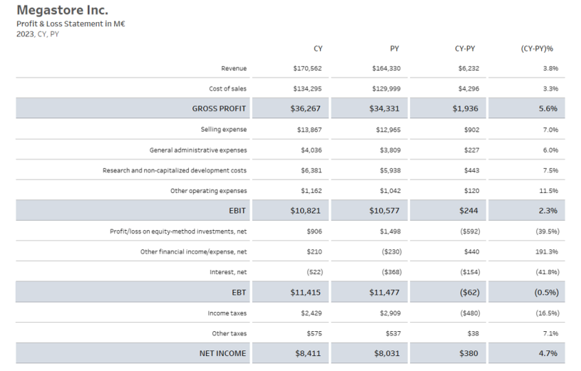
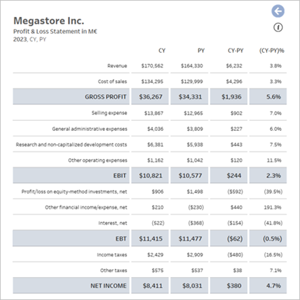
The aim of this blog is to offer a step-by-step explanation of the construction process for example number six, which can be found in “The Ultimate Profit & Loss Statement Workbook“.
This workbook was developed as part of “Tableau for Financial Reporting” initiative, a collaborative project that includes the contributions of Klaus Schulte, Annabelle Rincon, Steve Adams, and myself.
In this exercise we will put into practice the following:
- Customize the Subtotals name tag, without the need to duplicate the data.
- Customize whether, for display and presentation purposes in the P&L, the negative sign of negative amounts is shown or hidden.
- Customize the type of font to be used in the Subtotal rows.
- Customize the shading of the Subtotals rows.
- Add lines between the rows of the P&L.
The data source for the construction of this dashboard contains the following fields:

Next, I will share the steps to follow for its construction.
STEP 1. FORMULAS TO CUSTOMIZE THE SUBTOTAL LABELS.
Tableau allows us to define a generic label for the subtotal rows, however, for certain reports it is required to individually customize the label for each of the subtotals.
For this purpose, a frequently used solution involves duplicating the data, but there are also other techniques, perhaps not so widespread or well-known, that allow us to customize the subtotal labels without having to duplicate the data.
In this exercise we will put into practice one of these techniques, the first thing we must know is if the row shown is a subtotal or not.
One of the ways to know if it is a subtotal or not, is to calculate the number of different values of the dimensions of the hierarchy that are shown in the P&L.
The hierarchy in this example is made up of two dimensions “Sub-Total” and “Position”.
| 01.Level of Report | IIF(COUNTD([Position]) = 1, “1.Default”, IIF(COUNTD([Sub-Total]) = 1, “2.Subtotals”, “3.Grand Total”)) |
If the row you are displaying has a single element or value of the lowest level dimension (Position), it means that it is neither a subtotal nor a grand total and I will identify these rows as default rows.
If the previous condition is not met, it must be checked if the row that is being displayed has a single element or value of the largest dimension (Sub-Total), this means that it is a subtotal.
If neither of the two previous conditions is met, it implies that the row displayed is the grand total.
One condition for using this formula is that it requires each of the Sub-Totals in the report to contain two or more items from the bottom level of the data hierarchy (in this example, two or more values from the “Position” field) to that the formula can correctly identify that it is a Sub-Total row.
If the indicated condition is not met, a possible alternative would be to use the following formula:
| 01.Level of Report | IIF(SIZE() = 1, “3.Grand Total”, IIF(SIZE() =ATTR({COUNTD([Sub-Total])}), “2.Subtotals”, “1.Default”)) |
If you decide to use this option, you must bear in mind that the new formula requires checking that the “Size” value is not repeated between the different types of rows, to clearly identify the type of row.
I believe that in most cases, the conditions to use any of the two formulas interchangeably will be met, or failing that, they will be completed so that at least one of the two formulas can be used.
Returning to the exercise, since in this example we will not show (use) the grand total row, I decided to use a simplified version of the original formula.
| 01.Level of Report | IIF(COUNTD([Position]) = 1, “1.Default”, “2.Subtotals”) |
Once the level of detail of each row is known, the field for the personalized label can be defined.
| 02.Label | CASE [01.Level of Report] WHEN “1.Default” THEN ATTR([Position]) WHEN “2.Subtotals” THEN UPPER(ATTR([Sub-Total])) END |
Later, in the construction of the P&L, it will be explained how to show the labels in the P&L.
STEP 2. FORMULAS TO CUSTOMIZE THE SIGN OF THE NUMBERS.
From the very first examples that Klaus and I shared, we realized that we had different experiences/expectations regarding how signs should be presented in P&L reports.
For example, when dealing with a section that contained mixed concepts (such as a row for interest income and another row for interest expenses), I was used to the concepts of negative amounts (expenses) being presented with the negative sign, on the other hand, for Klaus, with the name of the concept was enough to identify if the amount was added or subtracted.
Given this exchange of experiences, we decided to try to make the calculations more flexible to find that they would adapt to the different requirements and in turn we expanded the examples, even in one of them, the negative sign is shown as part of the row label.
Returning to this exercise, as a first step we need to identify the specific accounting sections and/or concepts where negative amounts want to be presented as positive values in the P&L and that for practical purposes this translates to the amount being multiplied by -1 to convert the amount to a positive amount.
| 03.Sign | IIF([Position] = “Cost of sales” OR [Sub-Total] = “EBIT” OR [Sub-Total] = “Net Income”, -1, 1) |
It should not be forgotten that, although for presentation purposes a negative amount accounting concept must be shown as a positive value, for purposes of subtotal calculations, this concept must be accumulated as a negative amount. The following formula will make the adjustment for this consideration.
| 04.Sign by Level of Report | IIF([01.Level of Report] = “1.Default”, ATTR([03.Sign]), 1) |
STEP 3. FORMULAS OF THE AMOUNTS THAT WILL BE PRESENTED IN THE COLUMN.
Since we are working with a P&L, the subtotals are required to accumulate the amounts of the concepts previously presented, for which we will use the RUNNING_SUM() function.
| 05.CY | RUNNING_SUM(SUM([CY])) * [04.Sign by Level of Report] |
| 06.PY | RUNNING_SUM(SUM([PY])) * [04.Sign by Level of Report] |
| 07.CY-PY $ | RUNNING_SUM(SUM([CY] – [PY])) * [04.Sign by Level of Report] |
| 08.CY-PY % | RUNNING_SUM(SUM([CY] – [PY])) / ABS(RUNNING_SUM(SUM([PY]))) * [04.Sign by Level of Report] |
The RUNNING_SUM() table calculation must be defined to be calculated using the “Sub-Total” field so that the accumulation effect only applies to P&L subtotals.
The following table shows the different calculations of the “CY” field that are performed according to the level of the report.

STEP 4. FIELDS FOR GRAPH AXES.
These fields can be defined or captured directly in the row and/or column shelves within the sheet. This will create a (fake) axis.
| Axis | Date Measure | #1900-12-31# |
| Axis | Numeric Measure | 1.0 // Default Properties -> Aggregation -> Minimum (or Maximum or Average) |
| Row Axis | 1.0 // Default Properties -> Aggregation -> Minimum (or Maximum or Average) |
For the last two fields, the aggregation default property must be changed to “Minimum” (or Maximum or Average).
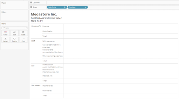
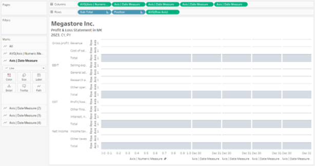
STEP 5. BUILD THE REPORT.
Add required fields to row and column shelves:
- Move the “Sub-Total” field to the rows shelf and sort ascending by the “Sub-Total No” field with minimum value aggregation.
- Move the “Position” field to the row shelf and sort ascending by the “Position No” field with minimum value aggregation.
- Change to line chart type, use white for color (#ffffff) with 0% opacity.
- Set the line size to the minimum.
- Activate the subtotals in the report (Menu “Analysis” -> “Totals” -> “Add all subtotals”.
- “Hide Field Labels for Rows”.
- Move the “Row Axis” field to the row shelf and set the range from 0 to 2.
- Add a reference line on this axis with a constant value of 2.
- A total of 5 columns will be defined and we will use a trick so that the first column that corresponds to the labels is wider. The first part of the trick involves defining the first column using a numeric type of field and the remaining columns must use a date type field.
- The first column will be used for the custom label.
- Move the field “Axis | Numeric Measure” to the row shelf and set the range from 0 to 1.
- The remaining four columns will be used to display the numerical values of the P&L.
- Move the field “Axis | Date Measure” and switch to handle “Exact Date” to the column shelf and set the range from “12/30/1900” to “12/31/1900”.
- Duplicate the field until completing the 4 date-type columns and establishing in each one the date ranges from “12/30/1900” to “12/31/1900”.
- The second part of the trick requires updating the configuration of the table options (Menu “Analysis” -> “Table Layouts” -> “Advanced” -> “Constrain aspect ratio 4 Horizontal: Vertical”.
- This will allow the first column to have a width of 4 to 1 concerning the remaining columns.
- You can try other ratios to adjust to your preference.
- The first column will be used for the custom label.

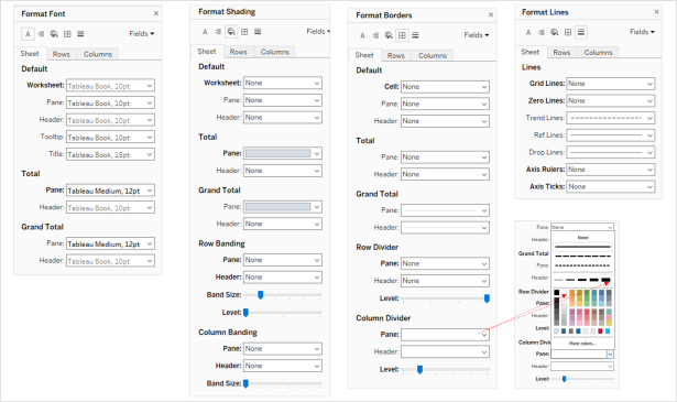
Adjust Formats:
- Format Font: For the default use “Tableau Book, 10pt” and for the subtotals use “Tableau Medium, 12 pt”.
- Shading Format: For the subtotals, the color #d6dce4 is used. For “Row Banding” and “Column Banding” the colors are removed.
- Format Borders: In “Row Divider” remove the line and in “Column Divider” establish a white line and select the thickest one.
- Format Lines: Set to “None” the “Grid Lines” and “Zero Lines”.
The grid can now be displayed.
Hide the “Sub-Total” and “Position” columns and hide the axes.
Add the fields to be displayed in each column to the text shelf and set text alignment to “Middle Right”. In case of numerical fields, adjust the table calculation to be calculated by the “Sub-Total” field.
- Column 1 -> Field “02.Label”
- Column 2 -> Field “05.CY”
- Column 3 -> Field “06.PY”
- Column 4 -> Field of “07.CY-PY $”
- Column 5 -> Field of “08.CY-PY%”
To simulate a margin to the right in the numerical columns, that is, from columns 2 to 5, the number format will be used: “$#,##0 ;(#,##0) ; “
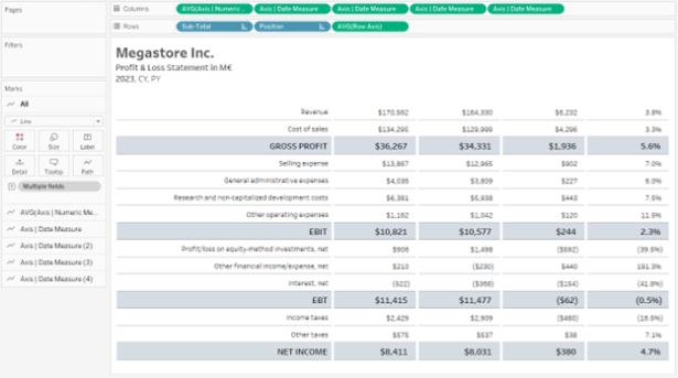
¡Ready!
Link here.

If you have any questions or comments about the exercise, please do not hesitate to get in touch.
